本コースの第3回目と第4回目では、NNgen とニューラルネットワーク・フレームワーク Pytorch を用いて、学習済みのモデルを SoC 型の FPGA の Ultra96-V2 上で動かしてみます。
今回の第3回では、学習済みモデルから FPGA のビットストリームを生成するところまで進めます。
環境構築
まずは、第1回ブログと同様に、NNgen を実行する環境を構築します。
- Ubuntu 18.04.4 LTS
- macOS 10.15.6 でも大丈夫です。
- Python: 3.7.7
- 任意の Python バージョンをインストールするには pyenv が便利です。
- Ubuntu 18.04 デフォルトの3.6系でも大丈夫です。
- Vivado: 2019.2
Vivado のインストール
Windows または Linux 環境に Vivado をインストールしましょう。ここでは2019.2を用います。
Icarus Verilog および Verilator のインストール
Ubuntu の場合、apt コマンドで Verilog シミュレータの Icarus Verilog と Verilator をインストールします。
sudo apt install iverilog verilatorPython の仮想環境の作成
システムデフォルトの Python 環境とは別に、Python の仮想環境を構築します。
mkdir nngen_test
cd nngen_test
python3 -m venv python3
source python3/bin/activate
もし、システムのデフォルトの Python 環境に戻る場合には、ターミナルのセッションを閉じるか、
deactivateと実行することで、仮想環境から抜けることができます。再度、仮想環境に戻る場合には、
cd nngen_test
source python3/bin/activate
としましょう。
依存ライブラリのインストール
作成した Python の仮想環境に以下の Python のライブラリをインストールします。
- veriloggen: 1.8.2
- pyverilog: 1.2.1
- pillow: 7.1.2
- onnx: 1.7.0
- torch: 1.5.0
- torchvision: 0.6.0
- jupyter: 1.0.0
Python の仮想環境上で、次のコマンドを実行します。
pip3 install veriloggen pyverilog pillow onnx torch torchvision jupyterNNgen のインストール
仮想環境上に NNgen をインストールします。第1回と同様に develop 版をインストールします。
git clone https://github.com/NNgen/nngen.git
cd nngen
python3 setup.py install
以上で、準備が整いました。
NNgen を用いて VGG-11 専用 IP コアを作る
今回は、画像分類に用いられる有名なニューラルネットワークモデルのひとつである、VGG-11 の専用ハードウェアを NNgen を用いて作成します。
本コースの第1回目では、NNgen のオペレータを組み合わせて、簡単なニューラルネットワークのモデルを構築しました。今回は、torchvision で提供される学習済みのモデルをハードウェアすることに挑戦します。もちろん、torchvision で提供されるモデルだけではなく、pytorch を用いてオリジナルのモデルを定義し学習することもできますが、今回は取り扱いません。
先ほど clone した NNgen のリポジトリに、torchvision の学習済みモデルをハードウェア化するサンプルがあるので、そのフォルダに移動しましょう。
cd nngen/examples/torchvision_onnx_vgg11ニューラルネットワークのモデルをハードウェア化するまでの流れを確認しましょう。テキストエディタで”torchvision_onnx_vgg11.py”を開き、run 関数の中を順番に追っていきましょう。
emacs torchvision_onnx_vgg11.py学習済みモデルのダウンロードと ONNX 形式への変換
torchvision から学習済みの VGG-11 のモデルをダウンロードし、変数 model に格納しています。バッチ正規化あり/なしの両方が提供されており、オプションでどちらを利用するか選択しています。その後、学習済みモデルを ONNX 形式でエクスポートします。
今回は学習済みモデルをダウンロードしていますが、もちろん、自前でモデルを定義の上学習してもかまいません。
    # input mean and standard deviation
    imagenet_mean = np.array([0.485, 0.456, 0.406]).astype(np.float32)
    imagenet_std = np.array([0.229, 0.224, 0.225]).astype(np.float32)

    act_shape = (1, 224, 224, 3)

    # pytorch model
    if with_batchnorm:
        model = torchvision.models.vgg11_bn(pretrained=True)
    else:
        model = torchvision.models.vgg11(pretrained=True)

    # Pytorch to ONNX
    dummy_input = torch.randn(*act_shape).transpose(1, 3)
    input_names = ['act']
    output_names = ['out']
    model.eval()
    torch.onnx.export(model, dummy_input, onnx_filename,
                      input_names=input_names, output_names=output_names)
ONNX 形式モデルを NNgen 形式へ変換する
ONNX 形式でエクスポートしたモデルを、NNgen 形式でインポートします。インポートする際に、活性値と重みなどのデータタイプ (ビット幅) を指定します。
    # --------------------
    # (1) Represent a DNN model as a dataflow by NNgen operators
    # --------------------

    # ONNX to NNgen
    dtypes = {}
    (outputs, placeholders, variables,
     constants, operators) = ng.from_onnx(onnx_filename,
                                          value_dtypes=dtypes,
                                          default_placeholder_dtype=act_dtype,
                                          default_variable_dtype=weight_dtype,
                                          default_constant_dtype=weight_dtype,
                                          default_operator_dtype=act_dtype,
                                          default_scale_dtype=scale_dtype,
                                          default_bias_dtype=bias_dtype,
                                          disable_fusion=disable_fusion)
モデルの量子化 (整数化)
NNgen で生成されるハードウェアアクセラレータは、整数 (固定小数) のみが利用できます。torchvision からダウンロードした学習済みモデルや、一般的なフローで学習したモデルは浮動小数を用いているため、量子化 (Quantization) により、整数化する必要があります。
量子化には、浮動小数で学習済みのモデルを量子化する方法 (Post-Training Quantization) と、量子化をしながら学習をする方法 (Quantization-Aware Training) の、大まかにわけて2つの方法があります。前者は、量子化を意識せずに学習したモデルを変換すればよいため、学習時に特別な処理を行う必要はなく手軽ではありますが、少ないビット数で数値を表現する場合には、認識精度が低下しやすいという欠点が存在します。後者は、学習時に量子化を適用して計算を行うために、計算グラフ定義に変更を加える手間はかかりますが、少ないビット数を用いる場合であっても、前者よりも高い精度を達成しやすいという利点が存在します。
NNgen は、学習済みのモデルをハードウェア化するコンパイラであるため、量子化を意識せずに学習されたモデルを量子化する、Post-Training Quantization のための量子化機能を搭載しています。整数化後は、乗算と加算を繰り返すのみでは、値の絶対値が増える傾向にあるため、適切な右シフト処理を挿入し、値を範囲を制御する必要があります。NNgen の量子化器では、想定される入力データの平均と分散に基づいて、ランダムに入力データを生成し、シフト量を決定します。ここでは、ImageNet のデータセットの平均と分散を用いています。
    # --------------------
    # (2) Assign quantized weights to the NNgen operators
    # --------------------

    if act_dtype.width > 8:
        act_scale_factor = 128
    else:
        act_scale_factor = int(round(2 ** (act_dtype.width - 1) * 0.5))

    input_scale_factors = {'act': act_scale_factor}
    input_means = {'act': imagenet_mean * act_scale_factor}
    input_stds = {'act': imagenet_std * act_scale_factor}

    ng.quantize(outputs, input_scale_factors, input_means, input_stds)
ハードウェアの並列化パラメータの設定
NNgen で生成されるハードウェアの並列性は、モデル定義とは別に、attribute という形で指定することができます。この例では、conv2d オペレータ (matmulオペレータを含む)、pool 系オペレータ、要素毎の演算 (ショートカットの加算等があれば) のそれぞれについて、並列度を指定しています。
    # --------------------
    # (3) Assign hardware attributes
    # --------------------

    for op in operators.values():
        if isinstance(op, ng.conv2d):
            op.attribute(par_ich=conv2d_par_ich,
                         par_och=conv2d_par_och,
                         par_col=conv2d_par_col,
                         par_row=conv2d_par_row,
                         concur_och=conv2d_concur_och,
                         stationary=conv2d_stationary)

        if isinstance(op, (ng.avg_pool, ng.max_pool,
                           ng.avg_pool_serial, ng.max_pool_serial)):
            op.attribute(par=pool_par)

        if ng.is_elementwise_operator(op):
            op.attribute(par=elem_par)
ソフトウェア実行による計算グラフの検証
第1回ブログと同様に、まずは量子化後の計算グラフが所望の動作をするか確認しましょう。NNgen 形式の計算グラフは、入力データを引数として渡すことで、量子化ハードウェア上での計算結果と同じ結果をソフトウェア実行で得ることができます。これにより、量子化により、最終的な認識までの振る舞いがどの程度変化するかをハードウェア化の前に確認できます。
まずは、Pytorch 上の浮動小数表現のモデルと NNgen 形式の整数表現モデルについて、最終出力および途中の各レイヤーの出力を取得します。入力には、同じフォルダにある写真画像を用いています。
    # --------------------
    # (4) Verify the DNN model behavior by executing the NNgen dataflow as a software
    # --------------------

    act = placeholders['act']
    out = outputs['out']

    # verification data
    img = np.array(PIL.Image.open('car.png').convert('RGB')).astype(np.float32)
    img = img.reshape([1] + list(img.shape))

    img = img / 255
    img = (img - imagenet_mean) / imagenet_std

    # execution on pytorch
    model_input = np.broadcast_to(img, act_shape)

    if act.perm is not None:
        model_input = np.transpose(model_input, act.reversed_perm)

    model.eval()
    model_out = model(torch.from_numpy(model_input)).detach().numpy()
    if act.perm is not None and len(model_out.shape) == len(act.shape):
        model_out = np.transpose(model_out, act.perm)
    scaled_model_out = model_out * out.scale_factor

    # software-based verification
    vact = img * act_scale_factor
    vact = np.clip(vact,
                   -1.0 * (2 ** (act.dtype.width - 1) - 1),
                   1.0 * (2 ** (act.dtype.width - 1) - 1))
    vact = np.round(vact).astype(np.int64)
    vact = np.broadcast_to(vact, act_shape)

    # compare outputs of hidden layers
    features_ops = [v for k, v in operators.items()
                    if isinstance(v, ng.conv2d) and not isinstance(v, ng.matmul)]
    features_ops = list(sorted(set(features_ops), key=features_ops.index))
    avgpool_op = [v for k, v in operators.items()
                  if isinstance(v, (ng.avg_pool, ng.avg_pool_serial))][0]
    classifier_ops = [v for k, v in operators.items() if isinstance(v, ng.matmul)]
    classifier_ops = list(sorted(set(classifier_ops), key=classifier_ops.index))

    sub_ops = features_ops + [avgpool_op] + classifier_ops
    sub_outs = ng.eval(sub_ops, act=vact)
    sub_outs = [sub_out.transpose([0, 3, 1, 2])
                for sub_out in sub_outs[:-len(classifier_ops)]] + sub_outs[-len(classifier_ops):]
    sub_scale_factors = ([features_op.scale_factor for features_op in features_ops]
                         + [avgpool_op.scale_factor]
                         + [classifier_op.scale_factor for classifier_op in classifier_ops])

    model.eval()
    model_features_relu_layers = [layer
                                  for layer in model.features if isinstance(layer, nn.ReLU)]
    model_features_relu_indexes = [list(model.features).index(layer)
                                   for layer in model_features_relu_layers]
    model_features_seqs = [model.features[:i + 1]
                           for i in model_features_relu_indexes]
    model_features_outs = [seq(torch.from_numpy(model_input)).detach().numpy()
                           for seq in model_features_seqs]

    model_avgpool_out = nn.Sequential(model.features,
                                      model.avgpool)(torch.from_numpy(model_input)).detach().numpy()

    class Flatten(nn.Module):
        def forward(self, input):
            return input.view(input.size(0), -1)

    model_classifier_relu_layers = [layer
                                    for layer in model.classifier if isinstance(layer, nn.ReLU)]
    model_classifier_relu_indexes = [list(model.classifier).index(layer)
                                     for layer in model_classifier_relu_layers]
    model_classifier_relu_indexes.append(len(model.classifier))
    model_classifier_seqs = [nn.Sequential(model.features, model.avgpool, Flatten(), model.classifier[:i + 1])
                             for i in model_classifier_relu_indexes]
    model_classifier_outs = [seq(torch.from_numpy(model_input)).detach().numpy()
                             for seq in model_classifier_seqs]

    model_outs = model_features_outs + [model_avgpool_out] + model_classifier_outs
    scaled_outs = [model_out * scale_factor
                   for model_out, scale_factor in zip(model_outs, sub_scale_factors)]

    max_diffs = [model_out.max() / sub_out.max()
                 for model_out, sub_out in zip(scaled_outs, sub_outs)]
    overflows = [np.sum(np.abs(sub_out) >= abs(2 ** (sub_op.dtype.width - 1) - 1))
                 for sub_op, sub_out in zip(sub_ops, sub_outs)]
    mean_square_errors = [np.sum((sub_out - model_out) ** 2) / sub_out.size
                          for model_out, sub_out in zip(scaled_outs, sub_outs)]
    corrcoefs = [np.corrcoef(model_out.reshape([-1]), sub_out.reshape([-1]))
                 for model_out, sub_out in zip(model_outs, sub_outs)]
最終出力および中間層の出力について、Pytorch 上での実行結果と NNgen のソフトウェア実行の結果を比較します。
    # compare prediction results
    eval_outs = ng.eval([out], act=vact)
    vout = eval_outs[0]

    mean_square_error = np.sum((vout - scaled_model_out) ** 2) / vout.size
    corrcoef = np.corrcoef(model_out.reshape([-1]), vout.reshape([-1]))

    class_index = json.load(open('imagenet_class_index.json', 'r'))
    labels = {int(key): value for (key, value) in class_index.items()}

    mout = scaled_model_out
    for bat in range(mout.shape[0]):
        m_top10 = list(sorted(enumerate(mout[bat]), key=lambda x: x[1], reverse=True))[:10]
        m_top10_indexes = [index for index, value in m_top10]
        v_top10 = list(sorted(enumerate(vout[bat]), key=lambda x: x[1], reverse=True))[:10]
        v_top10_indexes = [index for index, value in v_top10]
        num_hit = 0
        score = 0
        for index, value in m_top10:
            print("# mout: %s (%d) = %f" % (str(labels[index]), index, value))
        for index, value in v_top10:
            print("# vout: %s (%d) = %d" % (str(labels[index]), index, value))
            if index in m_top10_indexes:
                num_hit += 1
                score += 10 - abs(m_top10_indexes.index(index) - v_top10_indexes.index(index))
        print("# top-10 hit: %d" % num_hit)
        print("# top-10 score: %d" % score)
量子化の結果は、実行の都度変化するため、毎回同じ結果を得られるわけではありませんが、私の手元では以下のような結果が得られました。”mout”は Pytorch 上での浮動小数での実行結果、”vout”が量子化後の NNgen のソフトウェア実行での結果で、1000クラス分類における TOP-10 の推論結果をそれぞれ表示しています。今回は、活性値および重み共に、8ビットの量子化を適用していますが、ほとんど結果が変わらないことがわかります。この様子であれば、ハードウェア化しても問題なさそうです。
# mout: ['n04037443', 'racer'] (751) = 66.592598
# mout: ['n04285008', 'sports_car'] (817) = 61.874592
# mout: ['n03444034', 'go-kart'] (573) = 54.456955
# mout: ['n03895866', 'passenger_car'] (705) = 54.299454
# mout: ['n03770679', 'minivan'] (656) = 53.483257
# mout: ['n03670208', 'limousine'] (627) = 53.403870
# mout: ['n02930766', 'cab'] (468) = 53.018913
# mout: ['n03100240', 'convertible'] (511) = 50.271240
# mout: ['n02814533', 'beach_wagon'] (436) = 49.239208
# mout: ['n04461696', 'tow_truck'] (864) = 48.402401
# vout: ['n04037443', 'racer'] (751) = 63
# vout: ['n04285008', 'sports_car'] (817) = 57
# vout: ['n03444034', 'go-kart'] (573) = 52
# vout: ['n02930766', 'cab'] (468) = 48
# vout: ['n03100240', 'convertible'] (511) = 48
# vout: ['n03445924', 'golfcart'] (575) = 46
# vout: ['n03670208', 'limousine'] (627) = 46
# vout: ['n03770679', 'minivan'] (656) = 45
# vout: ['n03895866', 'passenger_car'] (705) = 45
# vout: ['n02814533', 'beach_wagon'] (436) = 44
# top-10 hit: 9
# top-10 score: 74
ハードウェアの生成
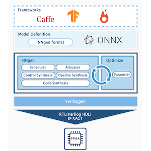
今回は Ultra96-V2 という ARM プロセッサを搭載する SoC 型の FPGA ボードを用いて、VGG-11 専用アクセラレータを開発します。”to_ipxact”関数で、IP-XACT 形式で IP コアを生成します。生成した IP コアは、本スクリプトと同じ、”nngen/examples/torchvision_onnx_vgg11″にあります。
    # --------------------
    # (5) Convert the NNgen dataflow to a hardware description (Verilog HDL and IP-XACT)
    # --------------------

    # to Veriloggen object
    # targ = ng.to_veriloggen([out], 'vgg11', silent=silent,
    #                        config={'maxi_datawidth': axi_datawidth})

    # to IP-XACT (the method returns Veriloggen object, as well as to_veriloggen)
    targ = ng.to_ipxact([out], 'vgg11', silent=silent,
                        config={'maxi_datawidth': axi_datawidth})

    # to Verilog HDL RTL (the method returns a source code text)
    # rtl = ng.to_verilog([out], 'vgg11', silent=silent,
    #                    config={'maxi_datawidth': axi_datawidth})
FPGA 実機で用いる量子化済みパラメータの保存
この後、実際のFPGA上で利用するニューラルネットワークの重みパラメータを、”export_ndarray”で単一の numpy の ndarray 形式へ変換し、ファイルとして保存します。NNgen で生成されるアクセラレータでは、すべての重みパラメータを並べた単一のバイナリデータを、予め指定のメモリ上に展開しておく必要があり、保存した重みパラメータファイルを、後程 FPGA の実機上で再度読み込みます。
    # --------------------
    # (6) Save the quantized weights
    # --------------------
    param_data = ng.export_ndarray([out], chunk_size)
    param_bytes = len(param_data)
    np.save(weight_filename, param_data)
FPGA のビットストリームを作る
続いて、NNgen で作成した VGG-11 専用の IP コアを搭載する FPGA ハードウェアを作ります。今回対象とする FPGA ボードは Xilinx Zynq UltraScale+ MPSoC ZU3EG を搭載する、Ultra96-V2 です。
以下の流れに従って、先ほど作った IP コアを CPU コア等と結合し、ハードウェア構成情報を生成しましょう。
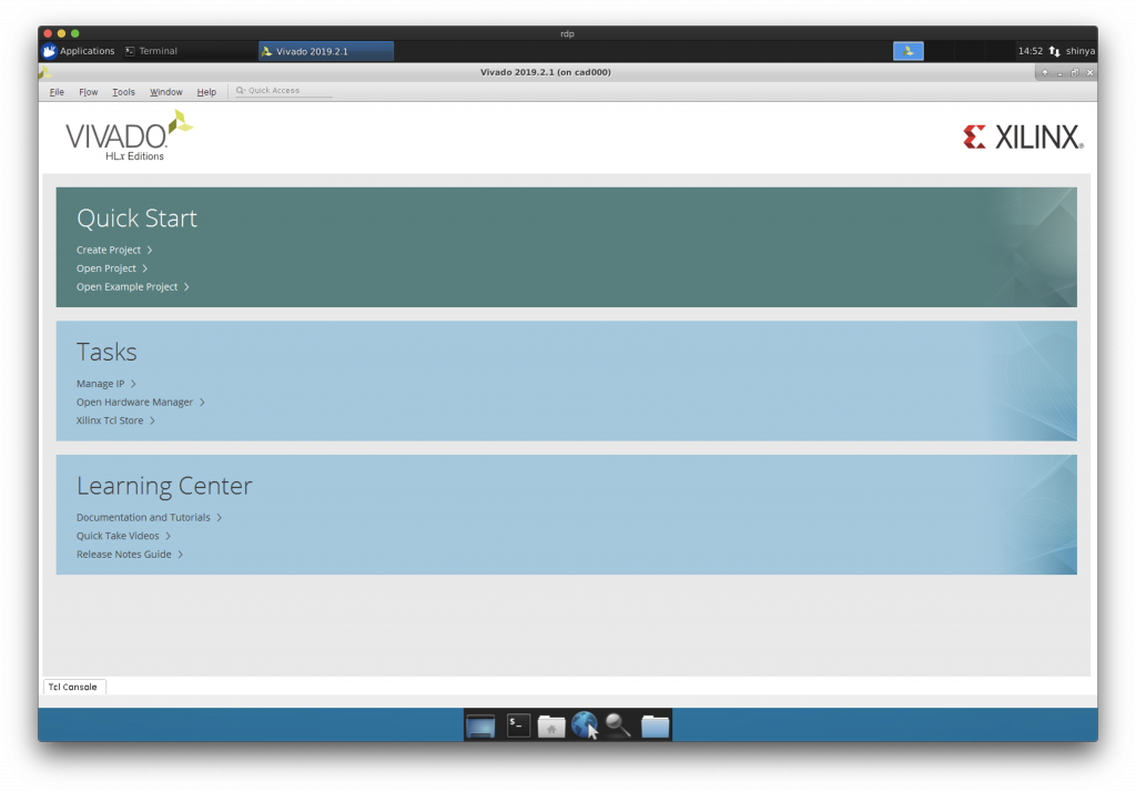
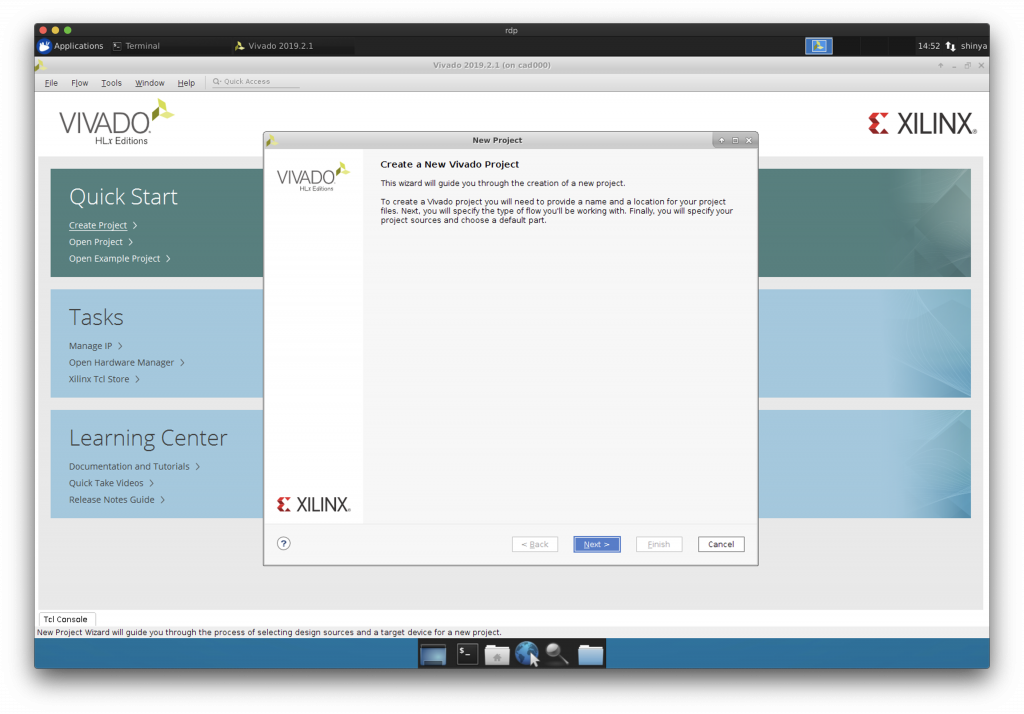
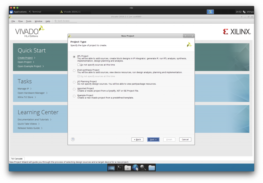
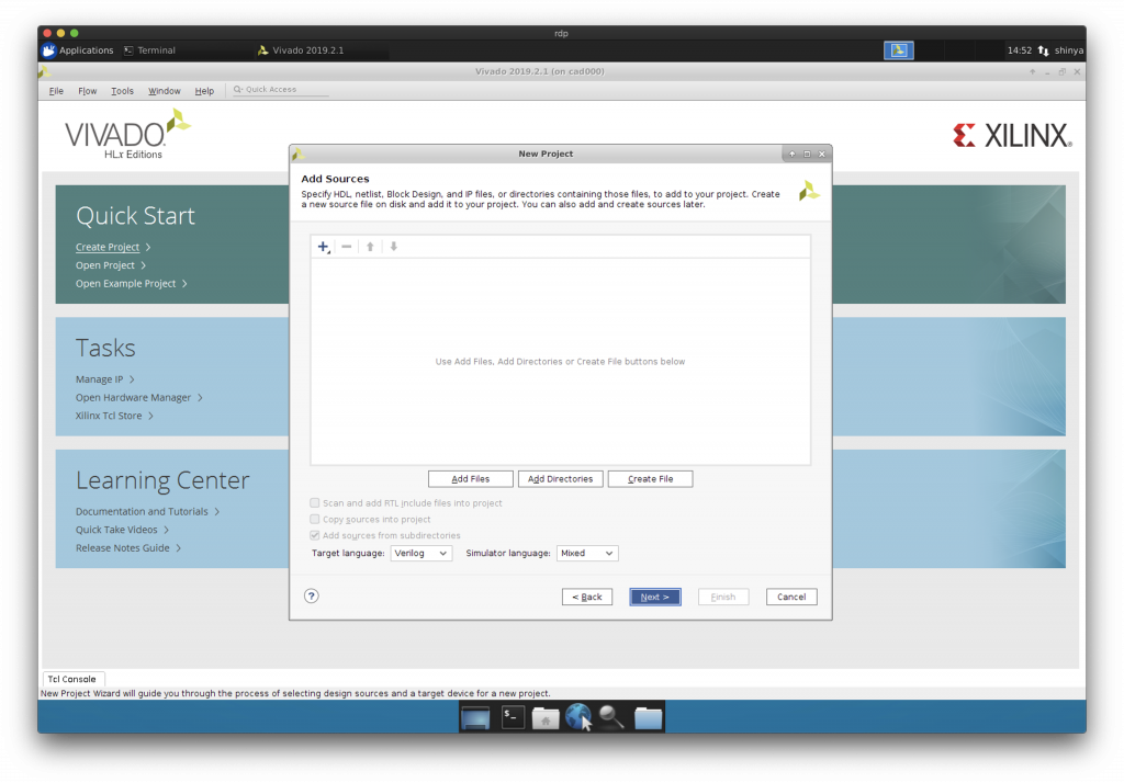
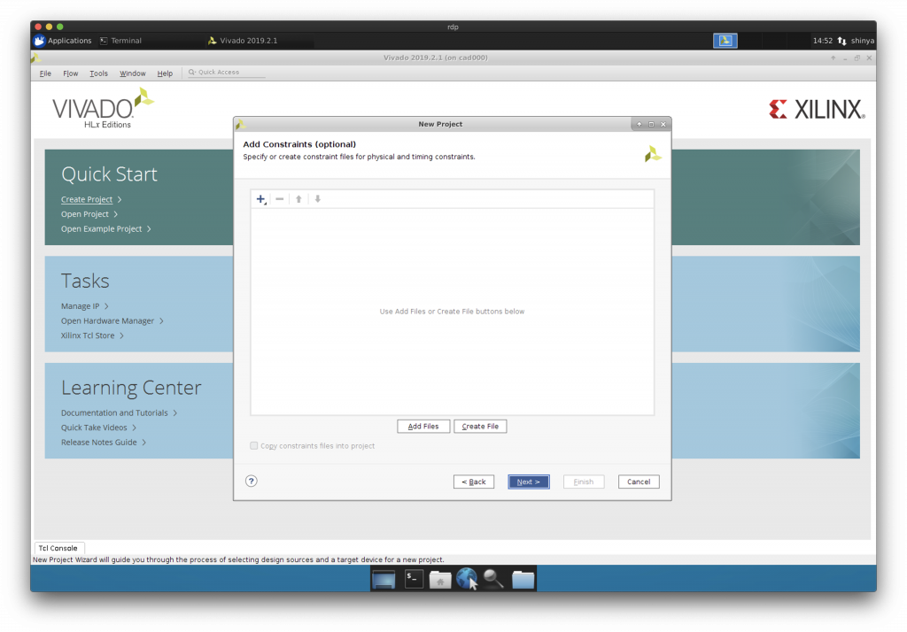
Vivado を立ち上げてプロジェクト作成
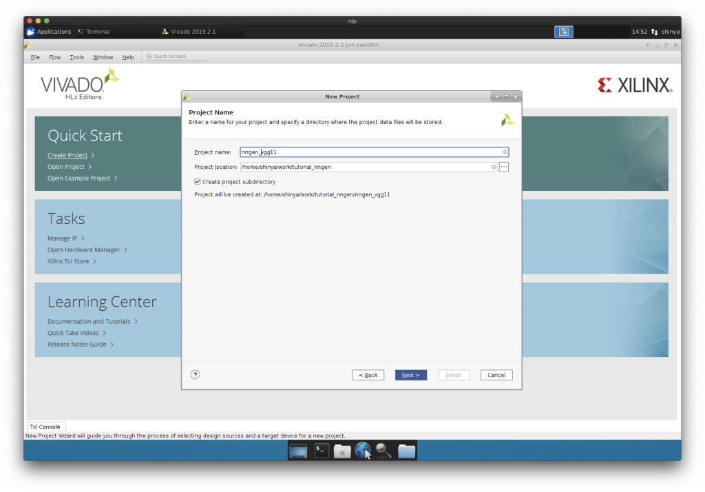
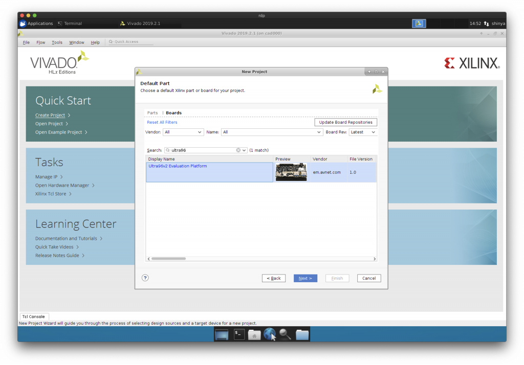
Default Part に Ultra96-V2 を選択します。
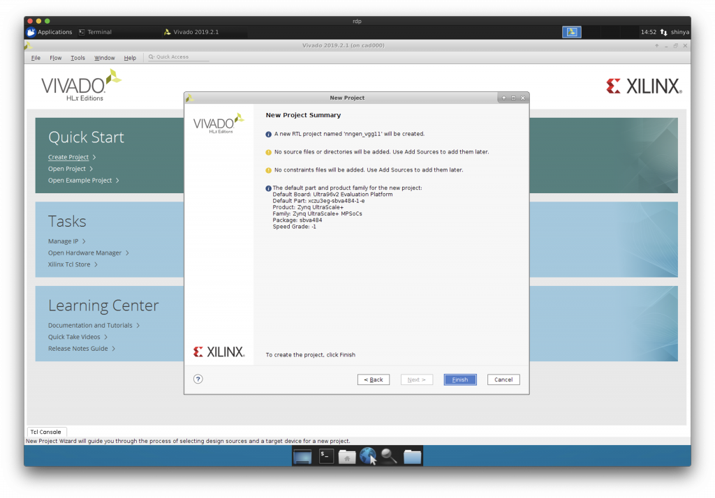
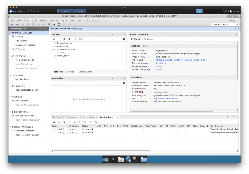
空のプロジェクトができました。
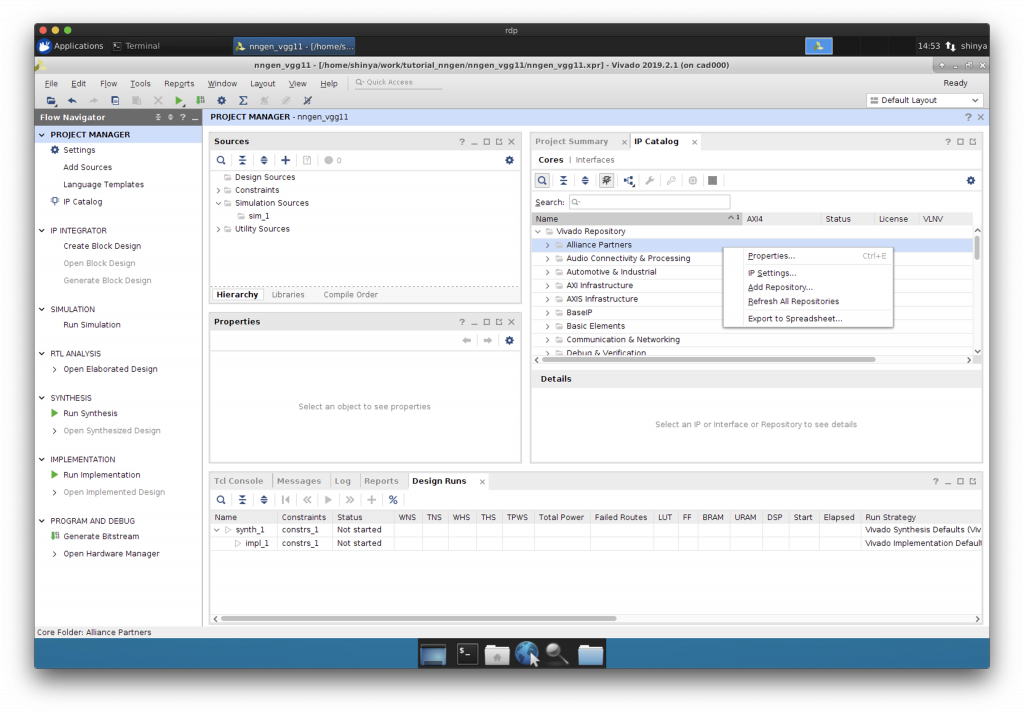
IP コアのリポジトリの追加
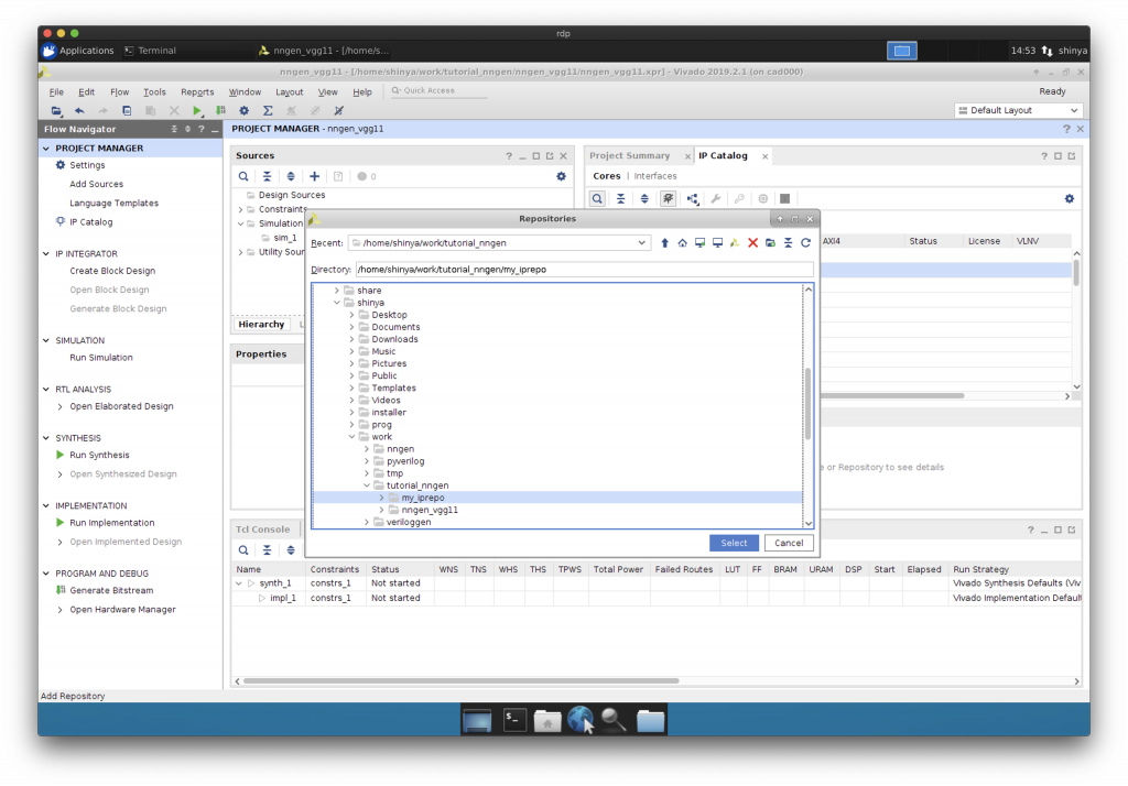
予め先ほど生成した IP コアを、どこか別の場所にコピーしておきましょう。この例では、”tutorial_nngen/my_iprepo”という場所にコピーしました。
“Add Repository”で IP コアがあるフォルダを IP コアのリポジトリとして追加します。
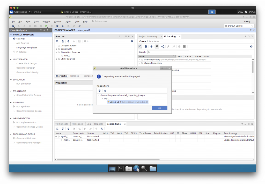
VGG-11 用の IP コアが認識されています。
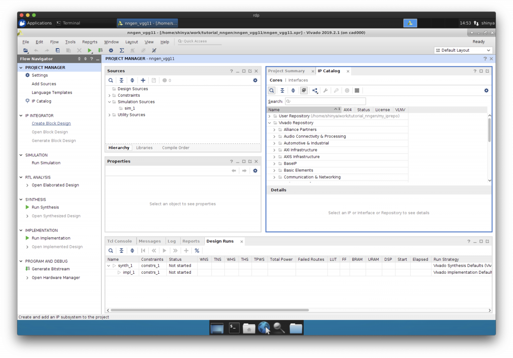
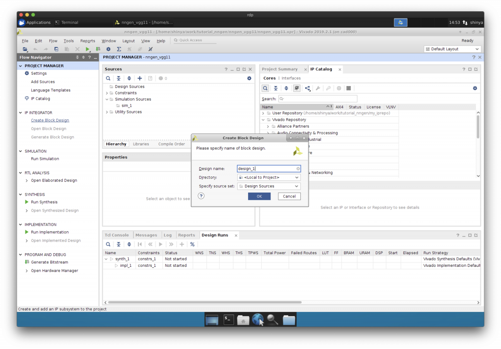
Block Design の作成
“Create Block Design”で新しい Block Design を作成します。
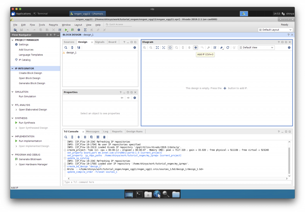
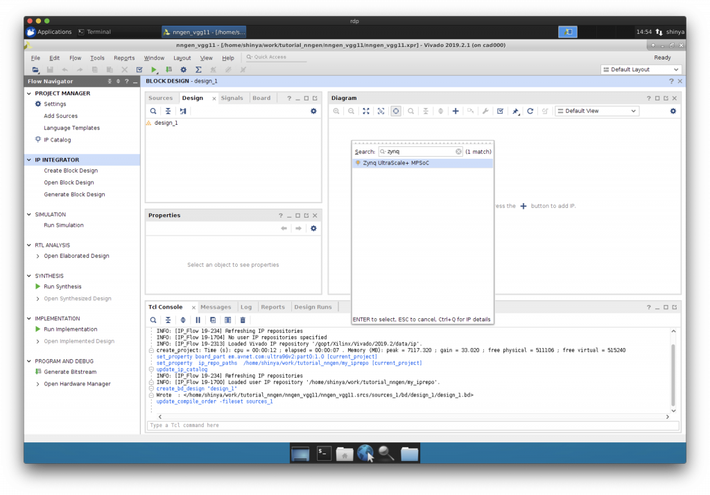
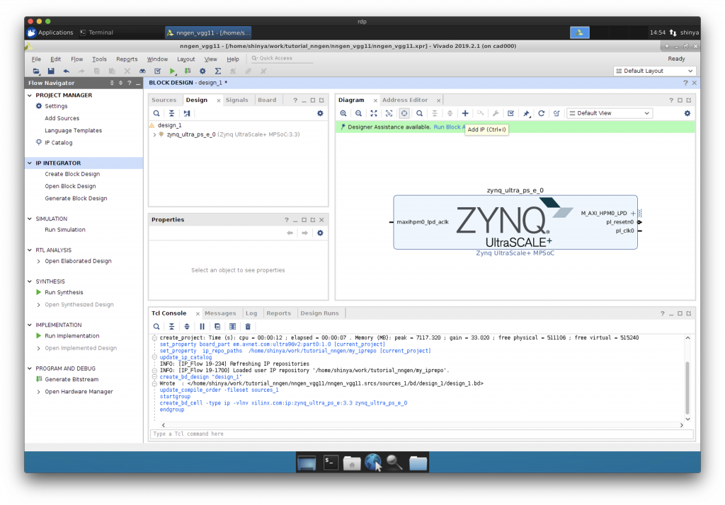
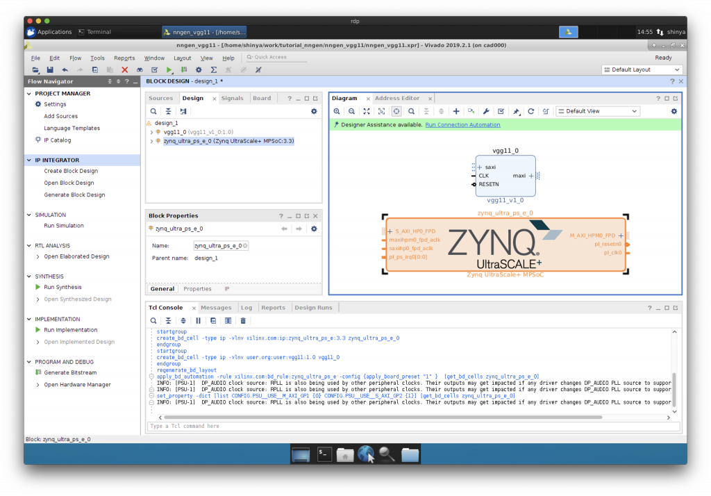
Block Design への CPU の追加
“Add IP”で Zynq に搭載されている ARM プロセッサを Block Design に追加します。
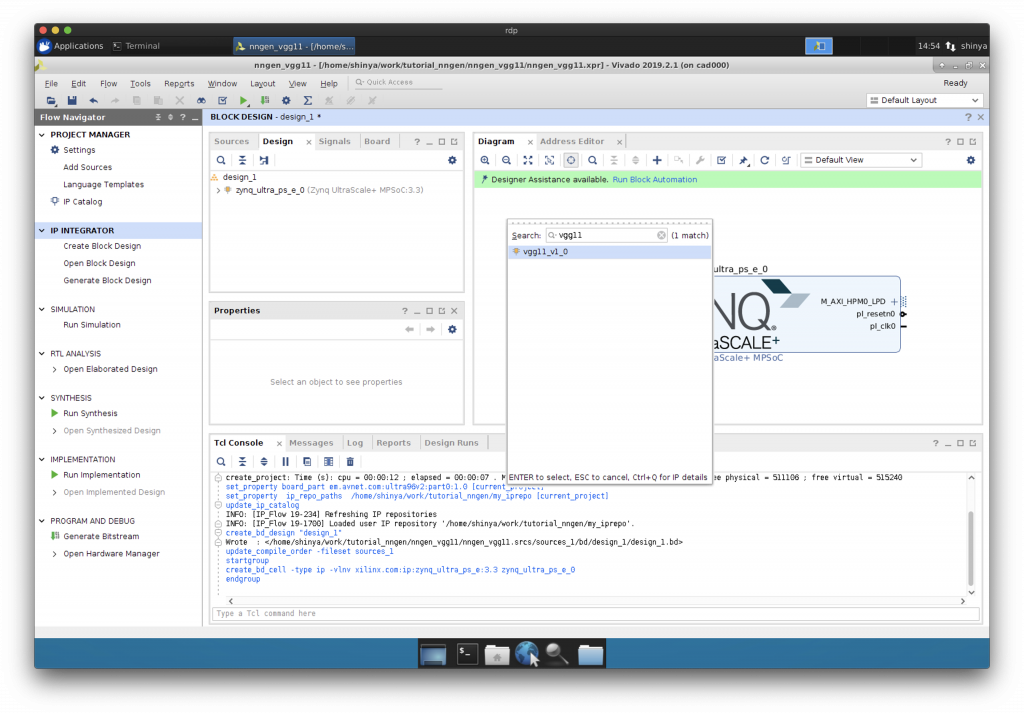
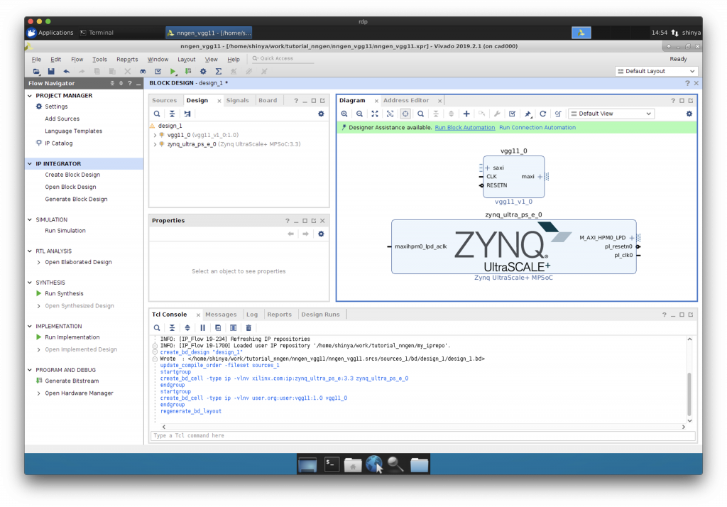
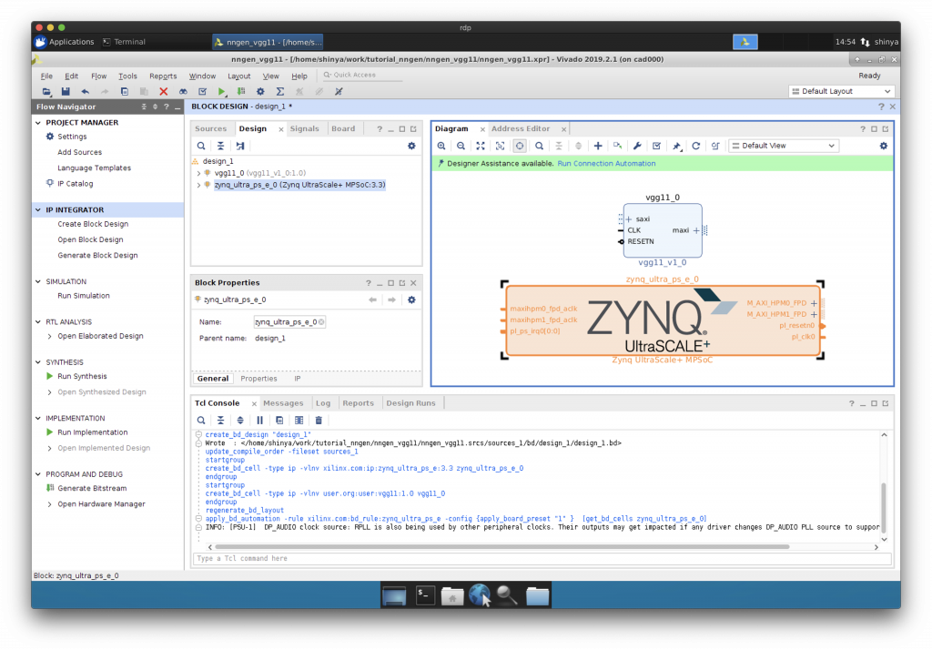
Block Design へのニューラルネットワークIPコアの追加
“Add IP”でニューラルネットワーク用の IP コアを Block Design に追加します。
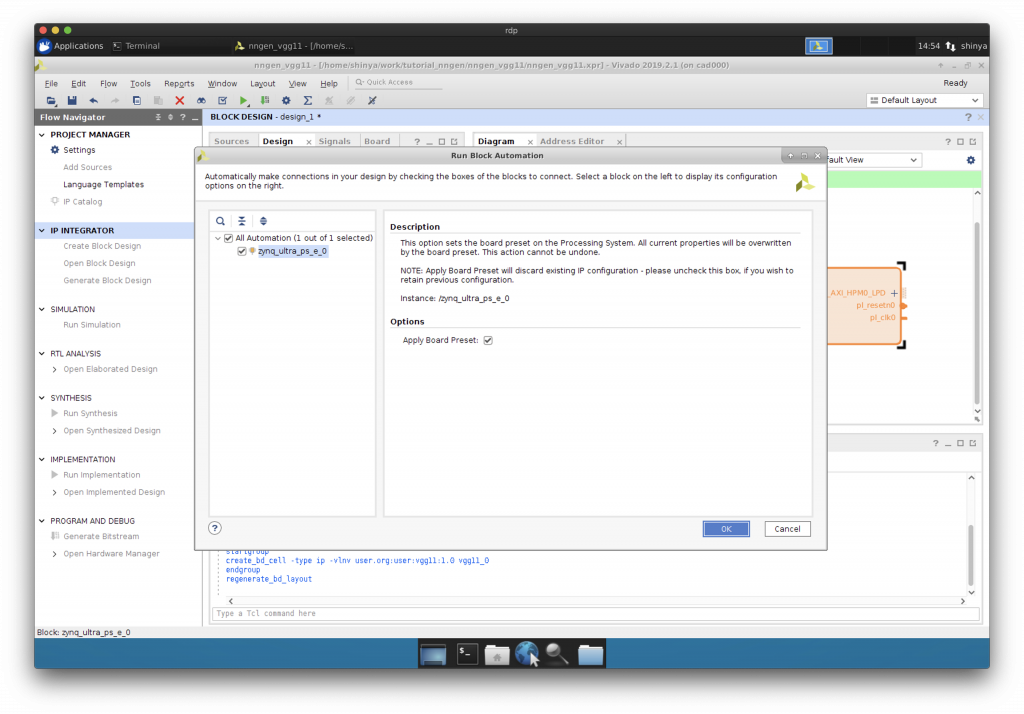
リセット信号の設定
“Run Block Automation”をクリックして、リセット信号の設定を行います。
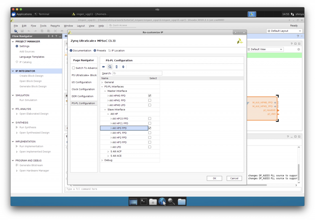
AXI HP ポートの追加
Zynq をダブルクリックして、AXI バスの HP ポートを追加します。
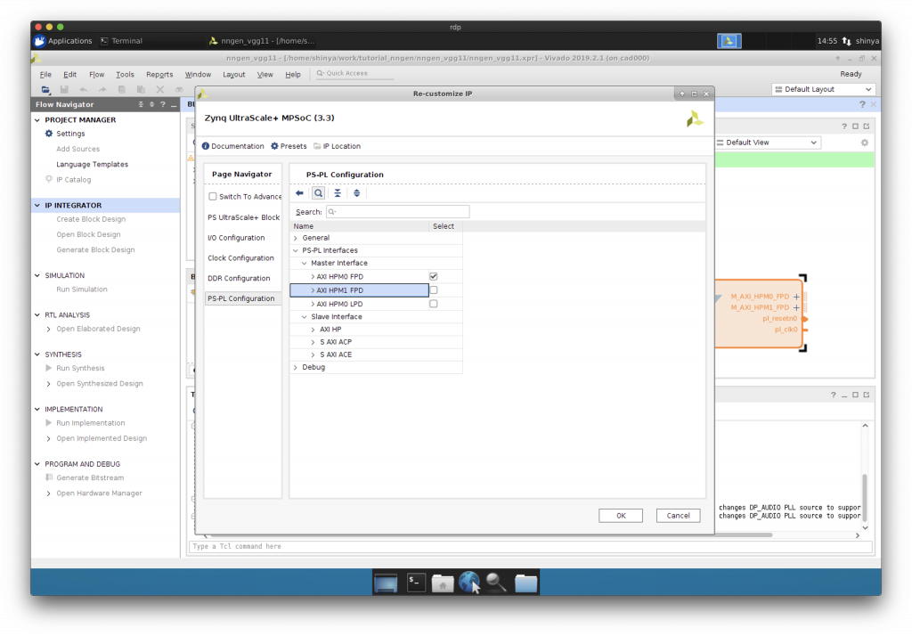
“AXI HP0 FPD”にチェックを入れます。
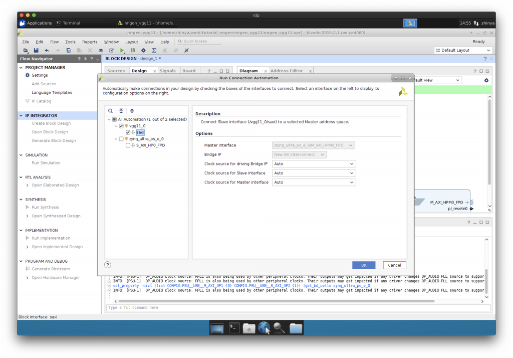
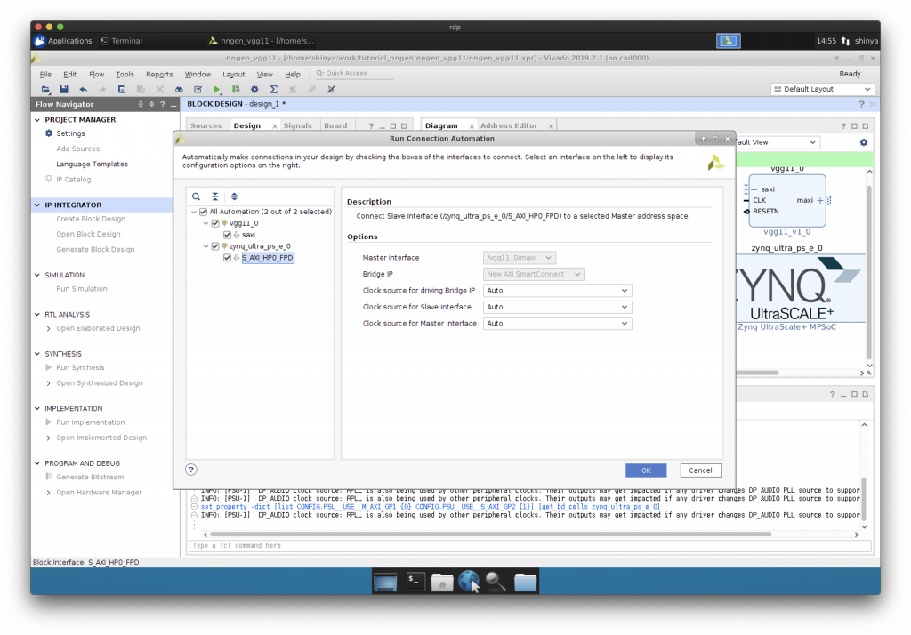
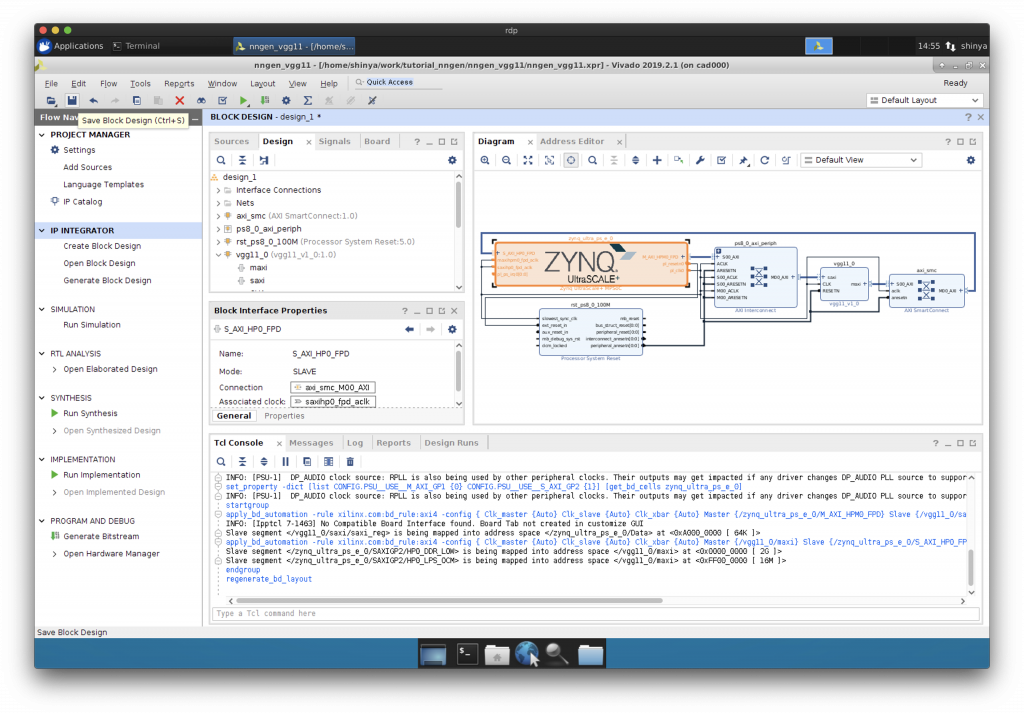
AXI を介した IP コアと CPU の接続
“Run Connection Automation”で CPU と IP コア等を AXI インターコネクトを介して接続します。
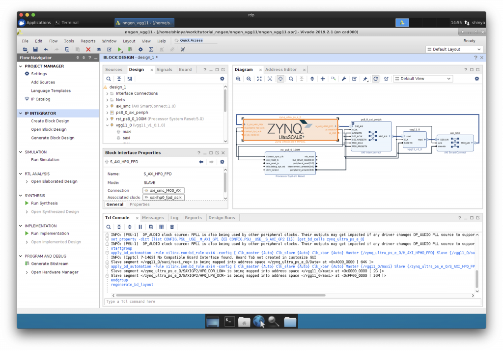
一旦、保存しておきましょう。
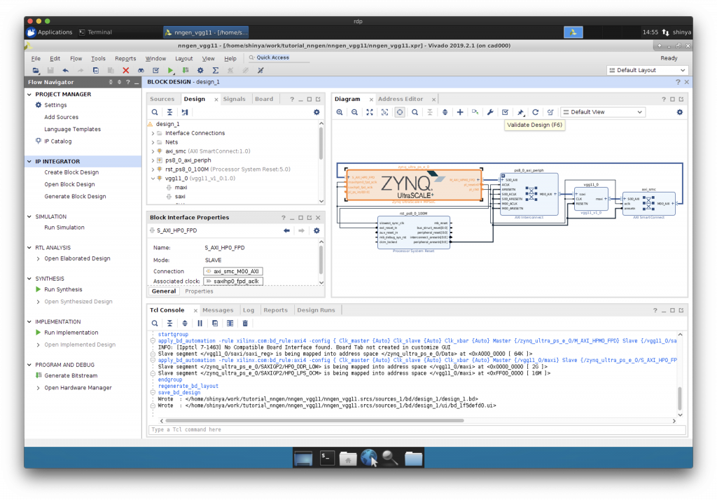
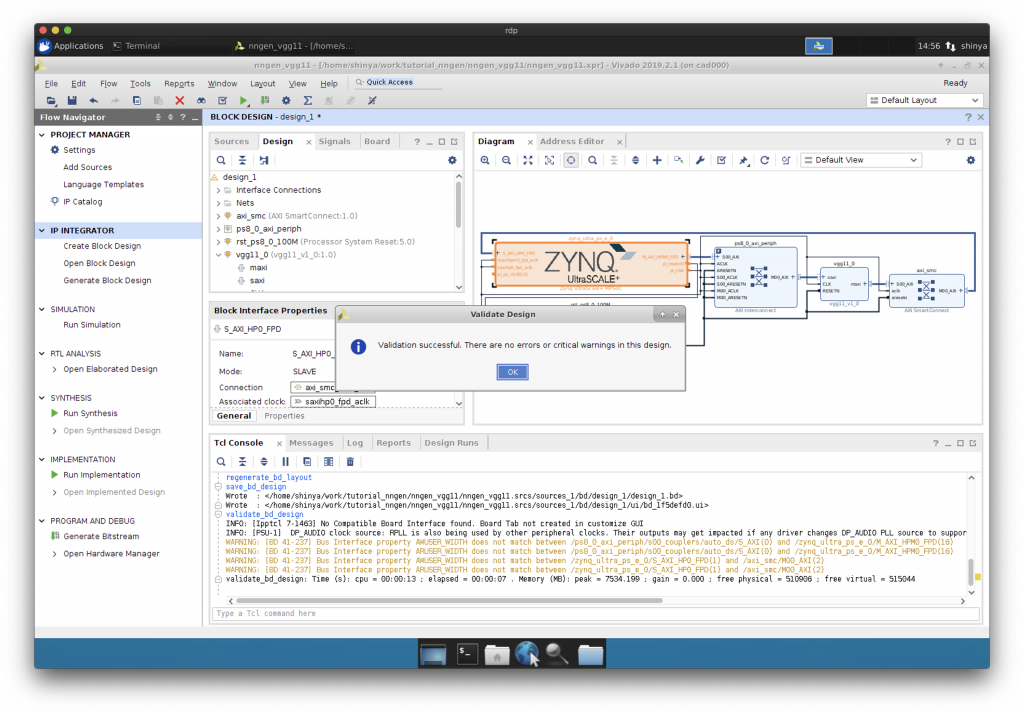
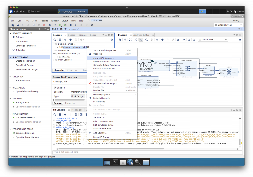
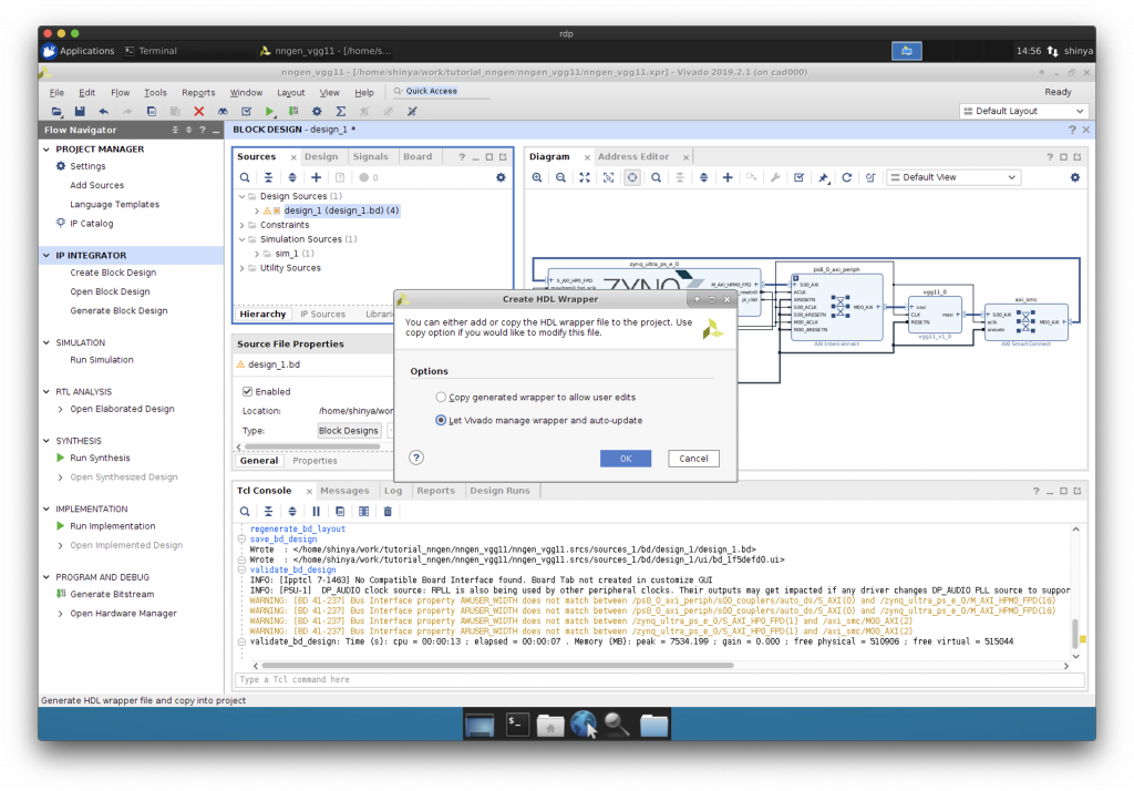
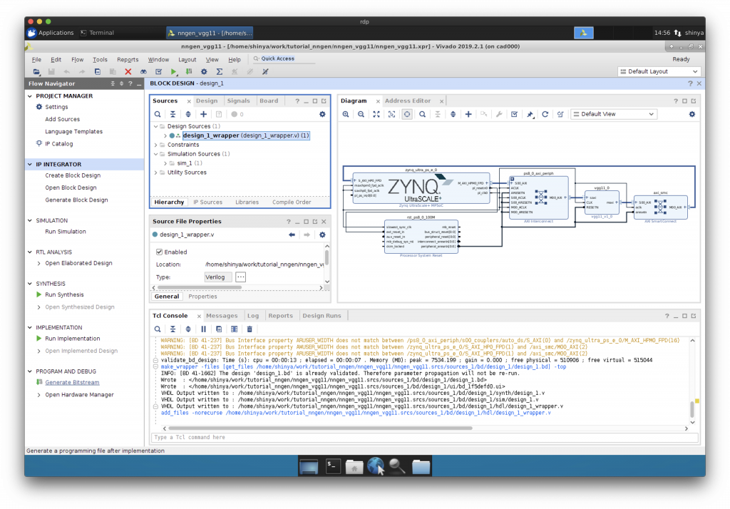
Validate してから、HDL Wrapper の作成
“Validate Design”で検証してから、HDL Wrapper を作成します。
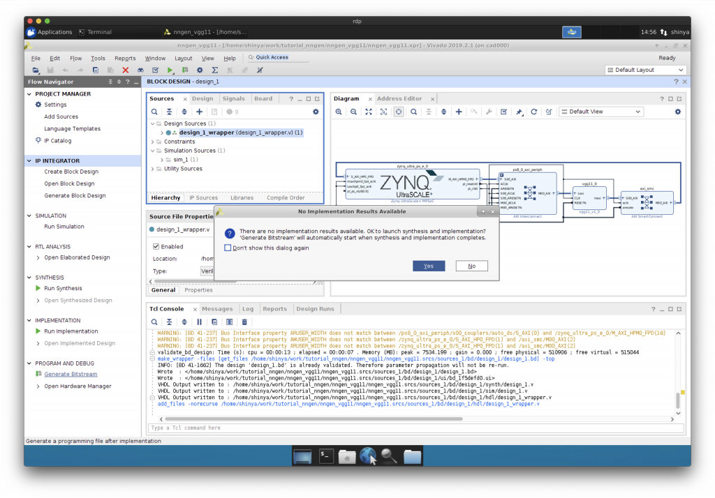
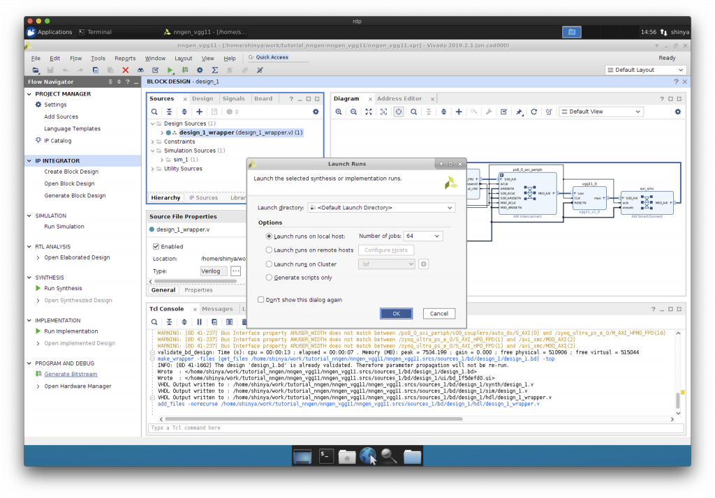
Synthesis, Implementation, Generate Bitstream
“Run Synthesis”, “Implementation”, “Generate Bitstream”と進めます。
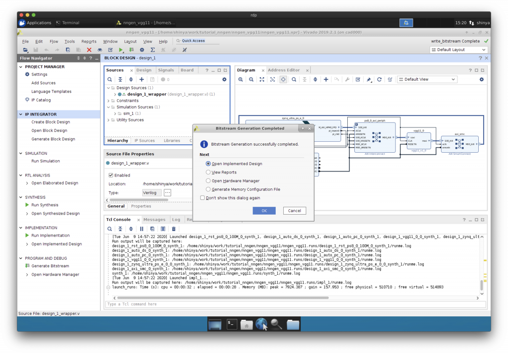
ビットストリームが完成しました。
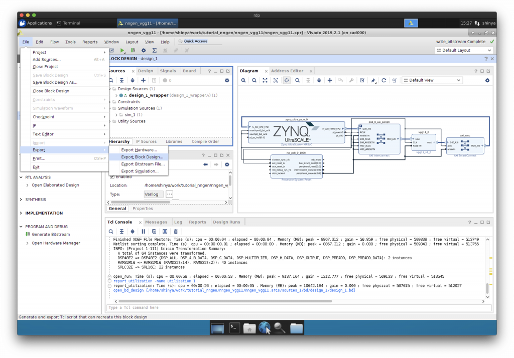
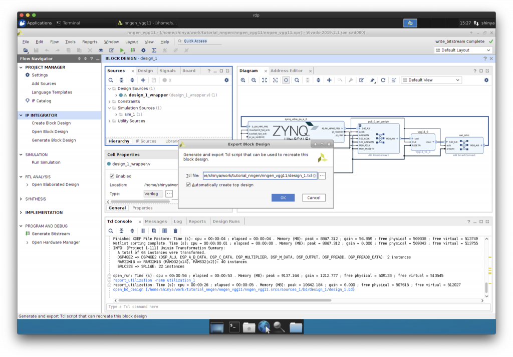
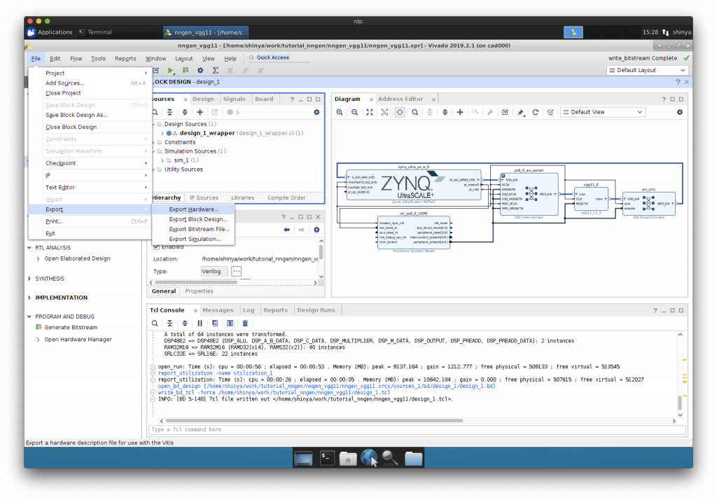
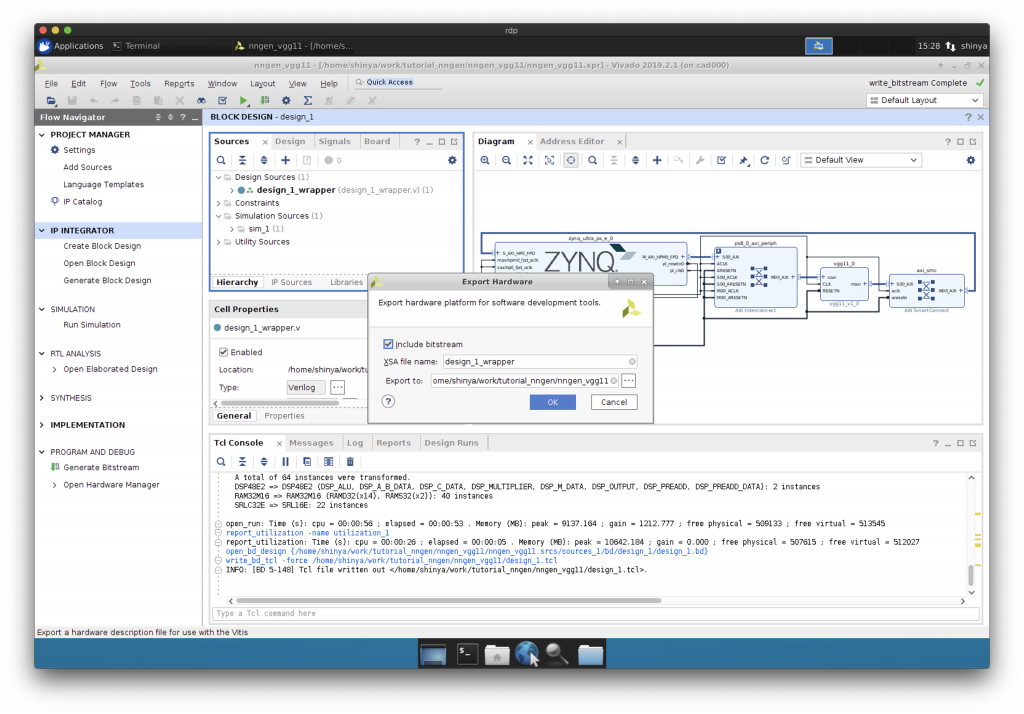
Export Block Design, Export Hardware
できあがったハードウェア情報のうち、後に PYNQ 上で必要になるファイルを保存します。
“Export Block Design”と”Export Hardware”を行います。
まとめ
これで VGG-11 の専用回路を搭載する FPGA アクセラレータのハードウェア構成情報が完成しました。次回は、PYNQ と Jupyter を用いて、今回開発した VGG-11 専用回路を実際の FPGA システム上で動かします。
東京大学 大学院情報理工学系研究科 コンピュータ科学専攻 高前田 伸也